Driver inference
The purpose of this part:
Retrieve potential drivers for a phenotype of interest and generate a master table of drivers.
A “lazy mode” function without flexible options is available for this part of the analysis: NetBID.lazyMode.DriverEstimation(). The user can find information about this function in manual and try using the demo code.
The complete step-by-step demo script for driver inference can be found here: pipeline_analysis_demo1.R.
Quick Navigation for this page
- Step 0: Preparations
- Step 1: Load in the expression dataset for analysis (exp-load, exp-cluster, exp-QC)
- Step 2: Read in network files and calculate driver activity (act-get)
- Step 3: Obtain differential expression (DE) / differential activity (DA) for drivers (act-DA)
- Step 4: Generate a master table for drivers (ms-tab)
Step 0: Preparations
Purpose: Create an organized working directory for the driver inference step in NetBID2 analysis.
Make sure that you have NetBID2 package.
library(NetBID2)
First, retrieve a constructed network for driver analysis. If the user has followed the Network reconstruction tutorial, the path of the network project network.dir should have been set. For details, please see Network reconstruction: Step 0. The network.project.name is used to distinguish different network reconstruction jobs when using SJAracne.prepare(), under the main path of network.dir. By specifying network.dir and network.project.name, the user should be able to retrieve the target network constructed by the network reconstruction part in NetBID2 and SJARACNe.
For the online tutorial, we have already prepared the demo dataset network constructed by SJARACNe. Therefore, the user does not need to run SJARACNe for the demo, and can proceed directly to the following pipeline.
network.dir <- sprintf('%s/demo1/network/',system.file(package = "NetBID2")) # use demo network in the package
network.project.name <- 'project_2019-02-14'
Next, create directories and folders to save and organize your analysis results.
We have designed a function NetBID.analysis.dir.create()to handle the working directories so that the user can have better data organization. Similar to the function in network reconstruction, this function needs the user to define the main working directory project_main_dir and the project name project_name. To prevent a previous project with the same project_main_dir and project_name from being rewritten, it is highly recommended that you add a time tag to your project_name.
# Define main working directory and project name
project_main_dir <- 'test/' # user defined main directory for the project, one main directory could
current_date <- format(Sys.time(), "%Y-%m-%d") # optional, if user like to add current date to name the project folder
project_name <- sprintf('driver_%s',current_date) # project name for the project folders under main directory
NetBID.analysis.dir.create() creates a main working directory with a subdirectory for the project. It also automatically creates three subfolders (QC, DATA and PLOT) within the project folder. QC/, storing Quality Control related plots; DATA/, saving data in RData format; and PLOT/, storing output plots. It also returns a list object, here named analysis.par with directory information wrapped inside. This list is an ESSENTIAL variable for the driver inference step, all of the important intermediate data generated later will be wrapped inside.
# Create a hierarchical working directory and return a list contains the hierarchical working directory information
# This list object (analysis.par) is an ESSENTIAL variable in driver inference pipeline
analysis.par  <- NetBID.analysis.dir.create(project_main_dir=project_main_dir, project_name=project_name,
                                            network_dir=network.dir, network_project_name=network.project.name)
Step 1: Load the expression dataset for analysis (exp-load, exp-cluster, exp-QC)
Purpose: Load the expression dataset for the driver inference analysis step.
For driver inference, we will need an expression dataset containing the phenotype of interest with proper control samples. In contrast to the dataset used for network reconstruction, there is no strong requirement for this dataset to have a large sample size. The user can choose to use the same dataset that was used for network reconstruction for this part, but this is not necessary. However, for the demo, we have chosen to use the same dataset. If the user chooses to use the same dataset, no pre-processing of the dataset is required. Because the expression dataset was saved after undergoing quality control as RData from the network reconstruction part, we can load it back directly. The user needs to assign network.par$net.eset to analysis.par$cal.eset, because for the driver inference step, the ESSENTIAL variable is analysis.par.
# If use the same expression dataset as in the network reconstruction, just reload it directly
load(sprintf('%s/DATA/network.par.Step.exp-QC.RData',network.dir)) # RData saved after QC in the network reconstruction step
analysis.par$cal.eset <- network.par$net.eset
If you choose to use a different dataset, please complete the first three steps in Network reconstruction first to process the dataset before performing further analysis.
For persistent storage of data and to prevent the re-running of all previous steps, the user can check out and save analysis.par as RData for this part. The function NetBID.saveRData() provides easier pipeline step checkout and reference. By giving the pipeline step name to step, the analysis.par will be saved with the step name as analysis.par$out.dir.DATA/analysis.par.Step.{exp-QC}.RData.
# Save Step 1 network.par as RData
NetBID.saveRData(analysis.par=analysis.par,step='exp-QC')
What do I do if the ID types from the network-reconstruction dataset and the analysis dataset are different?
-
It is highly recommended to use the ID type from the network-reconstruction dataset as the main ID type.
-
The purpose of NetBID2 is to find potential drivers in a biological process of interest based on the data-driven gene regulatory network. Each driver’s activity is evaluated based on the network structure (its directly targeted genes). If a driver does not exist in the pre-generated network, it will not be used in the activity calculation. In contrast, if a driver does not exist in the analysis dataset, its activity can still be calculated (if the expression values of its target genes are available).
-
We strongly recommend aligning the ID type from the analysis dataset to the network-reconstruction dataset by using
update_eset.feature(). The ID conversion table can be obtained from the GPL files or fromget_IDtransfer()andget_IDtransfer_betweenSpecies(). -
The most complicated situation is when the levels of the network-reconstruction ID type and the analysis expression dataset are different (e.g., the transcript level and the gene level are different). NetBID2 provides
update_eset.feature()to solve this problem by assigningdistribute_methodandmerge_methodparameters.
Step 2: Read in network files and calculate driver activity (act-get)
Please skip the following line if you did not close the R session after completing Step 1. Do not skip the line if you have checked out of and closed the R session after completing Step 1. Before starting Step 2, please reload the analysis.par RData from Step 1. NetBID.loadRData() reloads RData saved by NetBID.saveRData(). This prevents the user from repeating the previous pipeline steps. If the re-opened R session does not have analysis.par in the environment, please comment off the first two command lines. This will create a temporary analysis.par with the path of the saved Step 1 RData, analysis.par$out.dir.DATA. The path test//driver_2019-05-06//DATA/ is used here only as an example; the user needs to provide their own path that they used to save the analysis.par RData from Step 1.
# Reload network.par RData from Step 1
#analysis.par <- list()
#analysis.par$out.dir.DATA <- 'test//driver_2019-05-06//DATA/'
NetBID.loadRData(analysis.par=analysis.par,step='exp-QC')
Firstly, obtain the network constructed by SJARACNe. If you followed the pipeline, the file path should be analysis.par$tf.network.file and analysis.par$sig.network.file. Use get.SJAracne.network() to read in the network information. If you did not follow the pipeline, simply pass the directory of the network to get.SJAracne.network().
analysis.par$tf.network  <- get.SJAracne.network(network_file=analysis.par$tf.network.file)
analysis.par$sig.network <- get.SJAracne.network(network_file=analysis.par$sig.network.file)
More about get.SJAracne.network() and related function. This reads the SJARACNe network reconstruction result and returns a list object containing three elements: network_data, target_list and igraph_obj. network_dat is a data frame containing all of the information of the network constructed by SJARACNe. target_list is a driver-to-target list object. Please see details in get_net2target_list(). igraph_obj is an igraph object used to save this directed and weighted network. Each edge of the network has two attributes: weight and sign. The weight is the MI (mutual information) value, and the sign is the sign of the Spearman correlation coefficient (1, positive regulation; −1, negative regulation). To update the network dataset, the user can call update_SJAracne.network(). This updates the network object created by get.SJAracne.network, using constraints such as statistical thresholds and the list of genes of interest.
Generate an HTML QC report for the constructed network, using igraph_obj.
draw.network.QC(analysis.par$tf.network$igraph_obj,outdir=analysis.par$out.dir.QC,prefix='TF_net_',html_info_limit=FALSE)
draw.network.QC(analysis.par$sig.network$igraph_obj,outdir=analysis.par$out.dir.QC,prefix='SIG_net_',html_info_limit=TRUE)
Two QC reports have been created. One for the transcription factor TF network, the other is for the signaling factor SIG network.
- What information can you obtain from the HTML QC report of the network?
- A table for the network. This shows some basic statistics to characterize the target network, including the size and centrality, etc.
- A table of drivers. This shows detailed statistics for all drivers in the network.
- A density over histogram to show the distribution of the degree of nodes and the target size of all drivers. Experience suggests that an average target size of around several hundred may be preferable.
- A scatter plot to check whether the network is scale-free. It is helpful but not necessary for a gene regulatory network to have the scale-free topology feature.
Second, merge the TF network and the SIG network. There are two ways to merge the networks. (1) Merge the networks first by using merge_TF_SIF.network(), then calculate the activity value of the driver. (2) Calculate the activity values of the driver in the TF-network and the SIG-network, then merge them together by using merge_TF_SIG.AC(). Both approaches give the same result. Drivers in the analysis.par$merge.network will have the suffix “_TF” or “_SIG” to indicate their type. It is possible for a driver to have both “_TF” and “_SIG” suffixes.
# Merge network first
analysis.par$merge.network <- merge_TF_SIG.network(TF_network=analysis.par$tf.network,SIG_network=analysis.par$sig.network)
Third, obtain the activity matrix for all possible drivers by using cal.Activity(). The activity value of a driver quantifies its influence on a biological process. This is evaluated based on the accumulative effects of the driver on its targets. The evaluation strategies are “mean,” “weighted mean,” “maxmean,” and “absmean.” “Weighted mean” is the MI (mutual information) value with the sign of the Spearman correlation. For example, if the user chooses “weighted mean” to calculate the activity of a driver, then the higher the expression value of its positively regulated genes and the lower the expression value of its negatively regulated genes, the higher will be the activity value of that driver. If the user would like to perform a Z-transformation to the expression matrix before calculating the activity values, they can set std=TRUE.
# Get activity matrix
ac_mat <- cal.Activity(target_list=analysis.par$merge.network$target_list,cal_mat=exprs(analysis.par$cal.eset),es.method='weightedmean')
Now, we have an activity matrix ac_mat for drivers, in which the rows are drivers and the columns are samples. Because of the similar way in which the data is displayed and in which the phenotype information is shared, we can wrap the activity matrix into the ExpressionSet class object, just like an expression matrix.
# Create eset using activity matrix
analysis.par$merge.ac.eset <- generate.eset(exp_mat=ac_mat,phenotype_info=pData(analysis.par$cal.eset)[colnames(ac_mat),],
                                            feature_info=NULL,annotation_info='activity in net-dataset')
Fourth, create a QC report for the activity matrix. Use draw.eset.QC() to create the HTML QC report QC for AC of analysis.par$merge.ac.eset.
# QC plot for activity eset
draw.eset.QC(analysis.par$merge.ac.eset,outdir=analysis.par$out.dir.QC,intgroup=NULL,do.logtransform=FALSE,prefix='AC_',
             pre_define=c('WNT'='blue','SHH'='red','G4'='green'),pca_plot_type='2D.interactive')
Finally, save analysis.par. For persistent storage of data, and to prevent the re-running of all previous steps, the user can check out now and save analysis.par as RData for this part.
# Save Step 2 analysis.par as RData
NetBID.saveRData(analysis.par=analysis.par,step='act-get')
Why study driver activity ?
- Drivers, such as transcription factors (TFs) bind to the enhancer or promoter regions of their target genes and regulate their expression level. Once a TF has been synthesized, there are still many steps between mRNA translation of a TF and the actual transcriptional regulation of the target gene(s). The activity is controlled by most of the following processes: nuclear localization (importation into the cell nucleus), activation through signal-sensing domains (e.g., ligand binding or post-translational modifications such as methylation, ubiquitination, and phosphorylation, which is essential for dimerization and promoter binding), access to the DNA-binding site (involving epigenetic features of the genome), and interaction with other cofactors or TFs (to form complexes). Thus, the expression trend and the activity pattern of a driver may sometimes be contradictory. Because of these “hidden effects, analyzing the activity of a driver may be more fruitful than analyzing its expression level.
Step 3: Obtain differential expression (DE) / differential activity (DA) for drivers (act-DA)
Purpose: Obtain significantly differential expression (DE) and activity (DA) for all possible drivers in two phenotype groups.
Please skip the following line if you did not close the R session after completing Steps 1 and 2. Do not skip the line if you checked out of and closed the R session after completing Steps 1 and 2. Before starting Step 3, please reload the analysis.par RData from Step 2. NetBID.loadRData() reloads RData saved by NetBID.saveRData(). This prevents the user from repeating the previous pipeline steps. If the re-opened R session does not have analysis.par in the environment, please comment off the first two command lines. This will create a temporary analysis.par with the path of the saved Step 2 RData, analysis.par$out.dir.DATA. The path test//driver_2019-05-06//DATA/ is used here only as an example; the user needs to provide their own path that they used to save the analysis.par RData from Step 2.
# Reload network.par RData from Step 2
#analysis.par <- list()
#analysis.par$out.dir.DATA <- 'test//driver_2019-05-06//DATA/'
NetBID.loadRData(analysis.par=analysis.par,step='act-get')
Comparing driver activity in two phenotype groups. In the demo dataset, one column of the phenotype data frame is “subgroup”. This contains three phenotype groups: WNT, SHH and G4. To compare the differential expression (DE) and differential activity (DA) of a driver in any two groups (G1 vs. G0 in the following functions), NetBID2 provides two major functions getDE.BID.2G() and getDE.limma.2G(). The user needs to assign sample names from each group to G1_name and G0_name. In the script below, we compare G4.Vs.WNT and G4.Vs.SHH. Each comparison has a name (highly recommended, as it will be displayed in the final master table), and the results are saved in analysis.par$DE and analysis.par$DA.
More details. getDE.BID.2G() uses a Bayesian inference method to calculate DE and DA values by setting method='Bayesian'. If the user sets method='MLE', the calculation will take less time. If the input is RNA-seq dataset, the user can use the DE output from DESeq2. Just pay attention to the column names: one column should be Z-statistics. If the phenotype is ordinal or more complicated, the user can use bid() or limma() to analyze it.
# Create empty list to store comparison result
analysis.par$DE <- list()
analysis.par$DA <- list()

# First comparison: G4 vs. WNT
comp_name <- 'G4.Vs.WNT' # Each comparison must has a name
# Get sample names from each compared group
phe_info <- pData(analysis.par$cal.eset)
G1  <- rownames(phe_info)[which(phe_info$`subgroup`=='G4')] # Experiment group
G0  <- rownames(phe_info)[which(phe_info$`subgroup`=='WNT')] # Control group
DE_gene_bid <- getDE.BID.2G(eset=analysis.par$cal.eset,G1=G1,G0=G0,G1_name='G4',G0_name='WNT')
DA_driver_bid   <- getDE.BID.2G(eset=analysis.par$merge.ac.eset,G1=G1,G0=G0,G1_name='G4',G0_name='WNT')
# Save comparison result to list element in analysis.par, with comparison name
analysis.par$DE[[comp_name]] <- DE_gene_bid
analysis.par$DA[[comp_name]] <- DA_driver_bid

# Second comparison: G4 vs. SHH
comp_name <- 'G4.Vs.SHH' # Each comparison must has a name
# Get sample names from each compared group
phe_info <- pData(analysis.par$cal.eset)
G1  <- rownames(phe_info)[which(phe_info$`subgroup`=='G4')] # Experiment group
G0  <- rownames(phe_info)[which(phe_info$`subgroup`=='SHH')] # Control group
DE_gene_bid <- getDE.BID.2G(eset=analysis.par$cal.eset,G1=G1,G0=G0,G1_name='G4',G0_name='SHH')
DA_driver_bid   <- getDE.BID.2G(eset=analysis.par$merge.ac.eset,G1=G1,G0=G0,G1_name='G4',G0_name='SHH')
# Save comparison result to list element in analysis.par, with comparison name
analysis.par$DE[[comp_name]] <- DE_gene_bid
analysis.par$DA[[comp_name]] <- DA_driver_bid
Combining multiple comparison results. Wrap all of the comparison results into the DE_list, and pass it to combineDE(). This will return a list containing the combined DE/DA analysis. A data frame named “combine” inside the list is the combined analysis. Rows are genes/drivers, columns are combined statistics (e.g., “logFC,” “AveExpr,” “t,” and “P.Value”).
## Third comparison: G4 vs. others
# Combine the comparison results from `G4.Vs.WNT` and `G4.Vs.SHH`
comp_name <- 'G4.Vs.otherTwo' # Each comparison must has a name
DE_gene_comb <- combineDE(DE_list=list('G4.Vs.WNT'=analysis.par$DE$`G4.Vs.WNT`,'G4.Vs.SHH'=analysis.par$DE$`G4.Vs.SHH`))
DA_driver_comb <- combineDE(DE_list=list('G4.Vs.WNT'=analysis.par$DA$`G4.Vs.WNT`,'G4.Vs.SHH'=analysis.par$DA$`G4.Vs.SHH`))
analysis.par$DE[[comp_name]] <- DE_gene_comb$combine
analysis.par$DA[[comp_name]] <- DA_driver_comb$combine
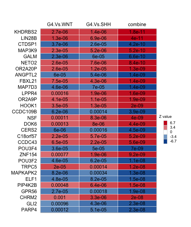
NetBID2 also provides draw.combineDE() to visualize the top drivers with significant DE/DA from the combined comparison, with DE/DA values from separate comparisons being listed as well. Drivers are sorted based on the P-values from the third column, which is the combined comparison (G4 vs. WNT+SHH).
- Driver table of top DE:
# Driver table of top DE
draw.combineDE(DE_gene_comb)
draw.combineDE(DE_gene_comb,pdf_file=sprintf('%s/combineDE.pdf',analysis.par$out.dir.PLOT)) # Save it as PDF
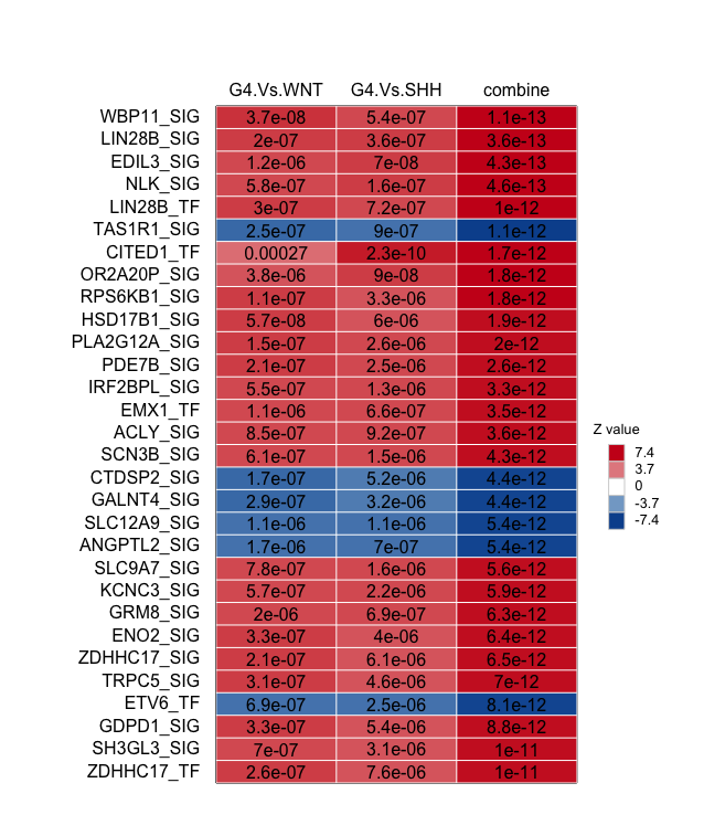
- Driver table of top DA:
# Driver table of top DA
draw.combineDE(DA_driver_comb)
draw.combineDE(DA_driver_comb,pdf_file=sprintf('%s/combineDA.pdf',analysis.par$out.dir.PLOT)) # Save it as PDF
Another way to perform the comparison of one group versus multiple groups is to choose the sample names from multiple groups as the G0_name parameter in the getDE.BID.2G(). In this way, the user does not need to call combineDE. However, the final result may vary because of the different statistical hypothesis.
# Another way to do the third comparison: G4 vs. others
comp_name <- 'G4.Vs.others'
# Get sample names from each compared group
phe_info <- pData(analysis.par$cal.eset)
G1  <- rownames(phe_info)[which(phe_info$`subgroup`=='G4')] # Experiment group
G0  <- rownames(phe_info)[which(phe_info$`subgroup`!='G4')] # Combine other groups as the Control group
DE_gene_bid <- getDE.BID.2G(eset=analysis.par$cal.eset,G1=G1,G0=G0,G1_name='G4',G0_name='others')
DA_driver_bid   <- getDE.BID.2G(eset=analysis.par$merge.ac.eset,G1=G1,G0=G0,G1_name='G4',G0_name='others')
# Save comparison result to list element in analysis.par, with comparison name
analysis.par$DE[[comp_name]] <- DE_gene_bid
analysis.par$DA[[comp_name]] <- DA_driver_bid
Save the comparison results as RData.
# Save Step 3 analysis.par as RData
NetBID.saveRData(analysis.par=analysis.par,step='act-DA')
We have now obtained the top differential expression (DE) and differential activity (DA) drivers from different comparisons. We can use draw.NetBID() to visualize the top drivers (the top 30 by default). Here, the displayed statistics for NetBID are set at P.Value and logFC for differential expression (set by DA_display_col and DE_display_col).
draw.NetBID(DA_list=analysis.par$DA,DE_list=analysis.par$DE,main_id='G4.Vs.others')
draw.NetBID(DA_list=analysis.par$DA,DE_list=analysis.par$DE,main_id='G4.Vs.others',pdf_file=sprintf('%s/NetBID_TOP.pdf',analysis.par$out.dir.PLOT),text_cex=0.8) # Save as PDF
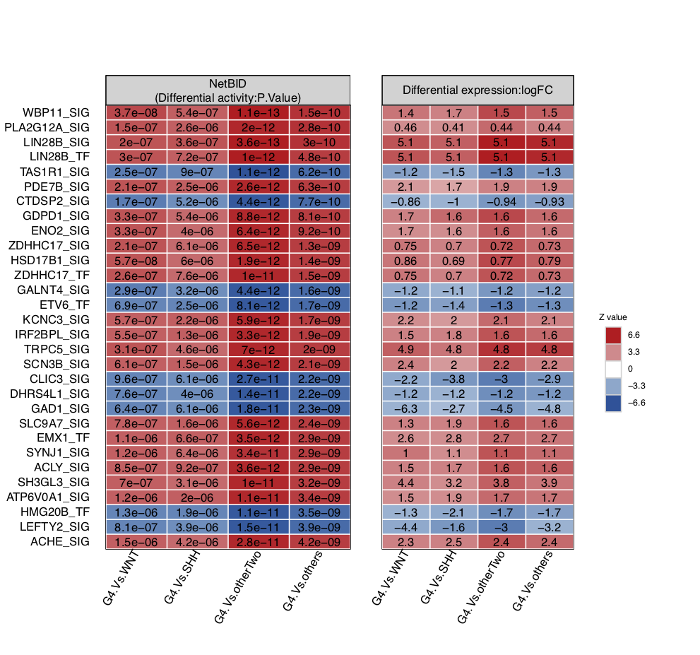
The user can customize the table above by choosing which column to display, i.e., DE or DA, or by choosing which comparison to display.
Step 4: Generate a master table for drivers (ms-tab)
Purpose: Gather the previously calculated data to create a final master table for all possible drivers.
Please skip the following line if you did not close the R session after completing Steps 1–3. Do not skip the line if you have checked out of and closed the R session after completing Steps 1–3. Before starting Step 4, please reload the analysis.par RData from Step 3. NetBID.loadRData() reloads RData saved by NetBID.saveRData(). This prevents the user from repeating the previous pipeline steps. If the re-opened R session does not have analysis.par in the environment, please comment off the first two command lines. This will create a temporary analysis.par with the path of the saved Step 3 RData, analysis.par$out.dir.DATA. The path test//driver_2019-05-06//DATA/ is used here only as an example; the user needs to provide their own path that they used to save the analysis.par RData from Step 3.
# Reload analysis.par RData from Step 3
#analysis.par <- list()
#analysis.par$out.dir.DATA <- 'test//driver_2019-05-06//DATA/'
NetBID.loadRData(analysis.par=analysis.par,step='act-DA')
To create the final master table, the user needs to gather the previous data and pass them to the parameters in the generate.masterTable() function. The details are as follows:
use_comp, the vector of multiple comparison names. This will be used for the columns of the master table. If all the comparisons are used, just callnames(analysis.par$DE).DEandDA: if following the previous pipeline, just useanalysis.par$DEandanalysis.par$DA.network,the driver-to-target list. The names of the list elements are drivers. Each element is a data frame, usually contains three columns: “target,” the target gene names; “MI,” the mutual information; and “Spearman,” the Spearman correlation coefficient. If following the previous pipeline, just useanalysis.par$merge.network$target_list.tf_sigs, contains all the detailed information on TFs and SIGs. The user needs to calldb.preload()for access.db.preload()reloads the TF/SIG gene lists into the R workspace and saves it locally under the db/ directory with the specified species name and analysis level.
z_col, the name of the column in thegetDE.limma.2G()andgetDE.BID.2G()output data frame that contains the Z-statistics. By default, it is “Z-statistics”.display_col,the statistical values of the other values for display. This must be columns from thegetDE.limma.2G()andgetDE.BID.2G()output data frame. For example, “logFC” and “P.Value”.main_id_type, the driver’s ID type. IMPORTANT. This comes from the attribute name in thebiomaRtpackage. Examples are “ensembl_gene_id”, “ensembl_gene_id_version”, “ensembl_transcript_id”, “ensembl_transcript_id_version” and “refseq_mrna”. For details, please see the ID conversion section.transfer_tab, the data frame for ID conversion. If NULL andmain_id_typeis not in the column names oftf_sigs, it will use the conversion table within the function. The user can also create their own ID conversion table. If the user wants to save it intoanalysis.par,we recommend callingget_IDtransfer2symbol2type()instead ofget_IDtransfer()as the output of the former function can be used in more visualization functions (e.gdraw.bubblePlot()).column_order_strategy, an option to re-order the columns in the master table. If set astype, the columns will be ordered by column type; if set ascomp, the columns will be ordered by comparison.
# Reload data into R workspace, and saves it locally under db/ directory with specified species name and analysis level.
db.preload(use_level='gene',use_spe='human',update=FALSE)
# Get all comparison names
all_comp <- names(analysis.par$DE) # Users can use index or name to get target ones
# Prepare the conversion table (OPTIONAL)
use_genes <- unique(c(analysis.par$merge.network$network_dat$source.symbol,analysis.par$merge.network$network_dat$target.symbol))
transfer_tab <- get_IDtransfer2symbol2type(from_type = 'external_gene_name',use_genes=use_genes)
analysis.par$transfer_tab <- transfer_tab
# Create the final master table
analysis.par$final_ms_tab <- generate.masterTable(use_comp=all_comp,DE=analysis.par$DE,DA=analysis.par$DA,
                                               target_list=analysis.par$merge.network$target_list,
                                               tf_sigs=tf_sigs,z_col='Z-statistics',display_col=c('logFC','P.Value'),
                                               main_id_type='external_gene_name')
Please note, Some drivers may have activity values but no expression values. This is because the network-reconstruction dataset differs from the analysis dataset.
Save the final master table as an EXCEL file. NetBID2 provides out2excel() to save the master table as an EXCEL file, with multiple options for highlighting data of interest (e.g., marker genes, drivers with significant Z-values). For more options, please see ?out2excel(). You can download the master table EXCEL file ms_tab.xlsx here.
# Path and file name of the output EXCEL file
out_file <- sprintf('%s/%s_ms_tab.xlsx',analysis.par$out.dir.DATA,analysis.par$project.name)
# Highlight marker genes
mark_gene <- list(WNT=c('WIF1','TNC','GAD1','DKK2','EMX2'),
                  SHH=c('PDLIM3','EYA1','HHIP','ATOH1','SFRP1'),
                  G4=c('KCNA1','EOMES','KHDRBS2','RBM24','UNC5D'))
# Customize highlight color codes
#mark_col <- get.class.color(names(mark_gene)) # this randomly assign color codes
mark_col <- list(G4='green','WNT'='blue','SHH'='red')
# Save the final master table as EXCEL file
out2excel(analysis.par$final_ms_tab,out.xlsx = out_file,mark_gene,mark_col)
We have now finished the driver inference part of NetBID2. We need to save the analysis.par as RData, because it contains all of the important results of the driver inference. This is ESSENTIAL to run the Advanced analysis part of NetBID2 and NetBID2 shiny server. The analysis.par list includes 13 elements (main.dir, project.name, out.dir, out.dir.QC, out.dir.DATA, out.dir.PLOT, merge.network, cal.eset, merge.ac.eset, DE, DA, final_ms_tab, and transfer_tab). These will be used to run NetBID shiny server.
# Save Step 4 analysis.par as RData, ESSENTIAL
NetBID.saveRData(analysis.par=analysis.par,step='ms-tab')
How to interpret and use the master table
out2excel()can save multiple master tables as excel sheets in one EXCEL file.- A master table consists of three parts:
- The first six columns are
gene_label,geneSymbol,originalID,originalID_label,funcTypeandSize.gene_labelis the gene symbol or transcript symbol of the driver, with the suffix “_TF” or “_SIG” to show the driver type.geneSymbolis the gene symbol or transcript symbol of the driver, without a suffix.originalIDis the original ID type used in the network reconstruction; it should match the ID type inanalysis.par$cal.eset,analysis.par$DE.originalID_labelis the original ID type with the suffix “_TF” or “_SIG”; it should match the ID type inanalysis.par$merge.network,analysis.par$merge.ac.eset,analysis.par$DA.originalID_labelis the only column to ensure an unique ID for a row record.funcTypeis either “TF” or “SIG” to indicate the driver type.Sizeis the number of target genes for the driver.
- The statistical columns are named as
prefix.comp_name_{DA or DE}. Theprefixcan beZ,P.Value,logFC, orAveExprto indicate which statistical value is stored. Thecomp_nameis the comparison name. For example,Z.G4.Vs.WNT_DAmeans the Z-statistics of the differential activity (DA) calculated from a comparison of the G4 and WNT phenotypes. The color of the background indicates the significance of the Z-statistics. - The next 13 columns (from
ensembl_gene_idtorefseq_mrna) contain detailed information for the genes. - The last columns (optional) contain the detailed information on marker genes; the user uses
mark_strategy='add_column'to set this column.
- The first six columns are
- The user can filter drivers by target size or sort the Z-statistics to obtain the top significant drivers. NetBID2 also provides Advanced analysis for advanced analysis and visualization.