Quick Tutorial for Running the Pipeline
Welcome to the Quick Tutorial for the bulk RNA-seq quantification pipeline! This tutorial aims to provide immediate and practical guidance for running this pipeline with your own data. As a quick tutorial, it is intended for users who are already familar with the basic concepts and tools of RNA-seq quantification analysis. If you are new to this field, we highly recommend starting with the Full Tutorial, which provides comprehensive documentation and step-by-step guidance.
To get started, activate the conda environment for this pipeline using the following commands:
module load conda3/202402 # conda version: 24.1.2
conda activate /research_jude/rgs01_jude/groups/yu3grp/projects/software_JY/yu3grp/conda_env/bulkRNAseq_2025
If you are using a different conda environment, please change the path accordingly. To set up a conda environment for this pipeline, please refer to the Pipeline Setup tutorial.
I. Prepare the sample table
The sample table is a table summarizing the essential information for all input samples required for quantification analysis. It serves as the central input file for the pipeline: every step of this pipeline is performed based on the entries in this table. Whether you have a single sample or thousands, you can list them all in this table. This is the only input file required to run this pipeline.
Below is an example of the sample table for this pipeline:
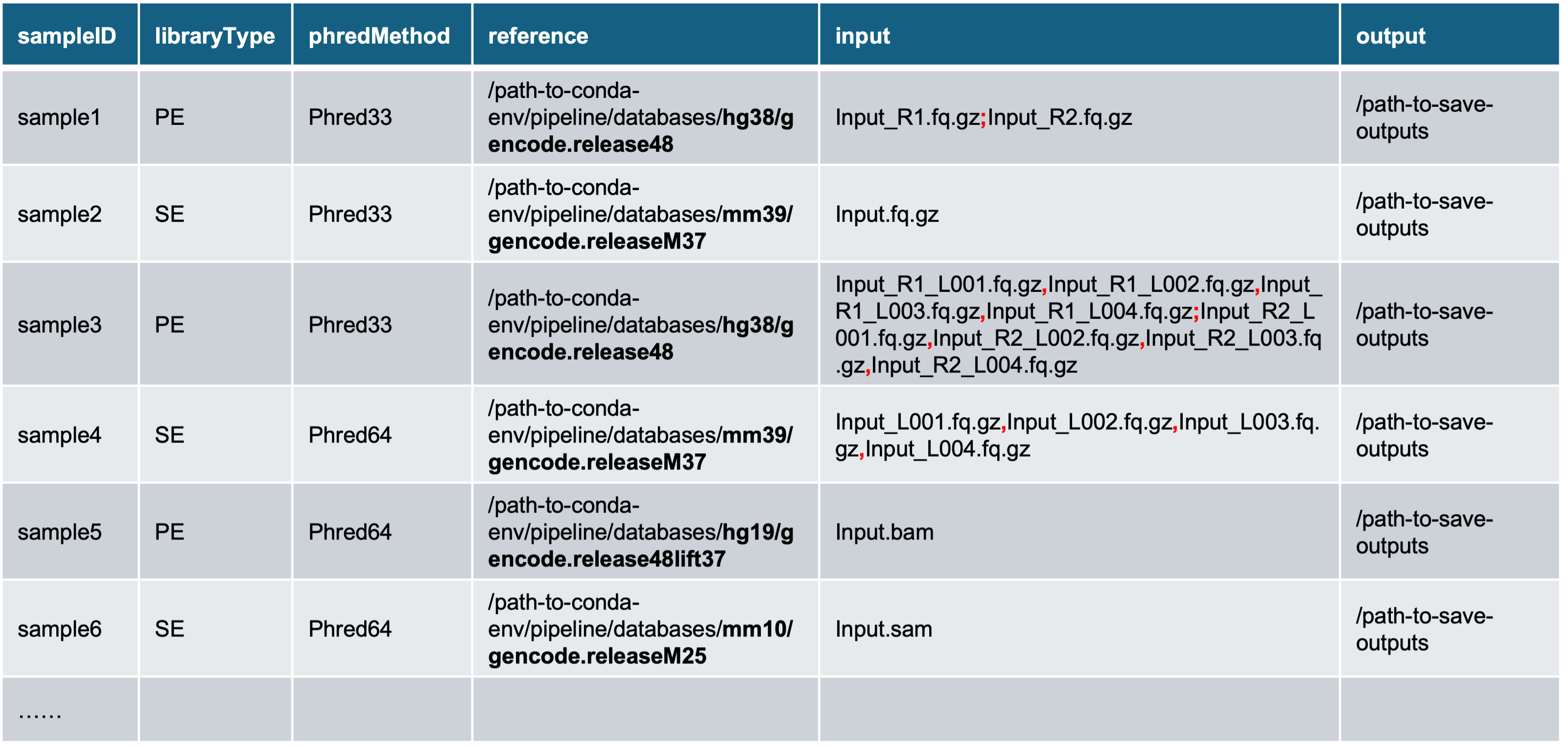
The sample table is a tab-delimited text file with 6 columns:
1) sampleID: name of samples. Some rules apply:
- Should contain letters, numbers or underscores ONLY;
- Should NOT start with numbers.
-
libraryType: type of libraries, paired-end or single-end,
[PE | SE].-
For BAM/SAM file inputs, not sure about their library type? You can use the command below to determine the library type:
## To tell the BAM/SAM files are single- or paired-end samtools view -c -f 1 input.bam # This command counts the matching records in the bam/sam file. # It returns 0 for single-end sequeing. Otherwise, the input bam/sam file is paired-end. # Loop over all BAM files in a directory for file in /path-to-directory/*.bam; do [ -e "$file" ] || continue # Skip if no matching files echo "Processing: $file" # Run samtools and capture output if output=$(samtools view -c -f 1 "$file" 2>/dev/null); then printf "$file\t$output\n" >> ./01_libraryType.txt else echo "Error processing $file" >&2 fi done -
For FASTQ file inputs, you typically have two paired files for
PEdata or one single file forSEdata. An exception, though exceedingly rare, is an interleaved FASTQ file, where both mate1 and mate2 reads are combined in a single file. This pipeline does not support interleaved FASTQ files as standard input. If you data is in this format, you will need to split it into two seperate FASTQ files before including them in your sample table.## To split an interleaved FASTQ file fastp --interleaved_in --in1 interleaved.fq --out1 fqRaw_R1.fq.gz --out2 fqRaw_R2.fq.gz # Then, use 'PE' as the library type and use 'fqRaw_R1.fq.gz' and 'fqRaw_R2.fq.gz' as the input in your sample table
-
-
phredMethod: Phred quality score encoding method,
[Phred33 | Phred64].Not sure about the answer? These two guidelines can help you determine the correct Phred encoding method:
-
Phred64 was retired in late 2011. Data genrated after that time should use Phred33.
-
You can use FastQC to identify the Phred encoding of your input files:
## To tell the Phred quality score encoding method in FASTQ/BAM/SAM files
# Method 1: use fastqc (good for small sample size)
fastqc input.fq.gz # for FASTQ files
fastqc input.bam # for BAM/SAM files
# This command generates a html report. In the "Basic Statistics" section, there is a measure called "Endcoding":
# "Sanger / Illumina 1.9" indicates Phred33, while "Illumina 1.5 or lower" indicates Phred64.

# Method 2: use samtools (good for large sample size, BAM files only)
samtools view input.bam | head -n 10000 | awk '{print $11}' | tr -d '\n' | od -An -t u1 | sed 's/\*//g' | awk '{for (i=1;i<=NF;i++) print $i}' | sort -n | awk 'NR==1{min=$1} {max=$1} END{print min,"\t",max}'
# This command prints two numbers: the first number indicates the smallest ASCII value of bases in top 10000 reads, while the sencond one indicates the largest ASCII value.
# Phred33 uses ASCII 33-126, while Phred64 uses 64-128.

# Loop over all BAM files in the current directory
for file in /path-to-directory/*.bam; do
	[ -e "$file" ] || continue # Skip if no matching files
  echo "Processing: $file"

  # Run samtools and capture output (from top 10000 reads)
	if output=$(samtools view "$file" | head -n 10000 | awk '{print $11}' | tr -d '\n' | od -An -t u1 | sed 's/\*//g' | awk '{for (i=1;i<=NF;i++) print $i}' | sort -n | awk 'NR==1{min=$1} {max=$1} END{print min,"\t",max}' 2>/dev/null); then
		printf "$file\t$output\n" >> ./02_phredScore.txt
	else
		echo "Error processing $file" >&2
	fi
done
-
-
reference: path to reference genome database folder. This pipeline contains four pre-built databases:
Genome Assembly Path hg38/GRCh38.p14 /research_jude/rgs01_jude/groups/yu3grp/projects/software_JY/yu3grp/conda_env/bulkRNAseq_2025/pipeline/databases/hg38/gencode.release48 hg19/GRCh37.p13 /research_jude/rgs01_jude/groups/yu3grp/projects/software_JY/yu3grp/conda_env/bulkRNAseq_2025/pipeline/databases/hg19/gencode.release48lift37 mm39/GRCm39 /research_jude/rgs01_jude/groups/yu3grp/projects/software_JY/yu3grp/conda_env/bulkRNAseq_2025/pipeline/databases/mm39/gencode.releaseM37 mm10/GRCm38.p6 /research_jude/rgs01_jude/groups/yu3grp/projects/software_JY/yu3grp/conda_env/bulkRNAseq_2025/pipeline/databases/mm10/gencode.releaseM25 If you are using a different conda environment, please change the paths accordingly. To set up a reference genome database, please refer to the Database Preparation tutorial.
- We recommend using
hg38for human samples andmm39for mouse samples. The other assemblies,hg19andmm10, are primarily intended for compatibility with legacy data. - If you cannot acccess to the paths listed above, or if you require other genome assemblies, you will need to manually create the reference files by following the Database Preparation tutorial.
- We recommend using
-
input: input files for quantification. This pipeline accepts the following formats:
-
Standard FASTQ files: both paired-end (e.g., sample1) and single-end (e.g., sample2). Filenames must be ended with
.fq,.fastq,.fq.gzor.fastq.gz. For paired-end samples, mate1 and mate2 should be catenated by *; (semicolon)*. -
FASTQ files of multple lanes: both paired-end (e.g., sample3) and single-end (e.g., sample4). Filenames must be ended with
.fq,.fastq,.fq.gzor.fastq.gz. The split FASTQ files of mate1 and mate2 must be listed in the same order and contenated using *, (comma)*. -
BAM/SAM files: alignment files with filenames ending in
.bam(e.g., sample 5) or.sam(e.g., sample6). Only one file per sample is accepted. If your sample consists of multiple BAM/SAM files (such as splited files), please merge them before proceeding:samtools merge -o merged.bam input_1.bam input_2.bam ...
-
-
output: the directory where output files will be saved. This pipeline will create a subfolder named by the
sampleIDwithin this directory.
Below are the two ways we recommend to generate the sample table:
-
Any coding language you prefer, e.g. BASH, R, Python, Perl et. al.
-
Excel or VIM. And for you convince, we have a templete avaible here:
/research_jude/rgs01_jude/groups/yu3grp/projects/software_JY/yu3grp/conda_env/bulkRNAseq_2025/pipeline/testdata/sampleTable.testdata.txt. You can simply copy it to your own folder and edit it using VIM. For those who can’t access to the path, download the template file here.
II. Data preprocessing
The purpose of data preprocessing is to prepare standard-in-format, clean-in-sequence FASTQ files that can be directly used for downstream quantification analysis. It consists of two steps:
-
Data format standardization: It converts input files, which may be in various formats (FASTQ, BAM, or SAM), into the standard FASTQ format.
-
Adapter trimming: It removes the adapeter sequences and low-quality bases from the reads.
1. Data format standardization
To standardize the data format, you can run the command below:
## 1. data format standardization
/research_jude/rgs01_jude/groups/yu3grp/projects/software_JY/yu3grp/conda_env/bulkRNAseq_2025/pipeline/scripts/run/all2Fastq.pl sampleTable.txt
This command will:
-
Create a folder,
sampleID/preProcessing, in the output directory specified by theoutputcolumn of sampleTable.txt. -
Generate the
sampleID/preProcessing/all2Fastq.shfile and submit it to HPC queues.
Typically, this step takes 5-10 mins to complete (for 150M PE-100 reads). The stardard outputs are:
- For PE library type: two paired FASTQ files,
sampleID/preProcessing/fqRaw_R1.fq.gzandsampleID/preProcessing/fqRaw_R1.fq.gz - For SE library type: one single FASTQ file,
sampleID/preProcessing/fqRaw.fq.gz
2. Adapter trimming
You can perform the adapter trimming analysis by:
## 2. adapter trimming
/research_jude/rgs01_jude/groups/yu3grp/projects/software_JY/yu3grp/conda_env/bulkRNAseq_2025/pipeline/scripts/run/adapterTrimming.pl sampleTable.txt
This command will:
- Generate the
sampleID/preProcessing/adapterTrimming.shfile and submit it to HPC queues.
Typically, this step takes ~5 mins to complete (for 150M PE-100 reads). The stardard outputs are:
- adapter trimming reports in differnt formats:
sampleID/preProcessing/adapterTrimming.htmlandsampleID/preProcessing/adapterTrimming.json - standard FASTQ files with clean/filtered sequences:
- For PE library type: two paired FASTQ files,
sampleID/preProcessing/fqClean_R1.fq.gzandsampleID/preProcessing/fqClean_R1.fq.gz - For SE library type: one single FASTQ file,
sampleID/preProcessing/fqClean.fq.gz
- For PE library type: two paired FASTQ files,
After completing these two preprocessing steps, you will have standard FASTQ files with clean sequences that are ready to be used in subsequent quantification analysis.
III: Quantification
Though there are five quantification methods (see the table below) available in this pipleline, we use Salmon and RSEM_STAR as the default ones:
- Salmon: a wicked-fast alignment-free method. Its accuracy has been further enhanced with the introduction of decoy sequences. *Salmon can automatically determine the strandness of your data, and this information will be utilized by other methods*. These features make it an excellent complement to alignment-based methods for cross-validation purpose.
- RSEM_STAR: an alignment-based method. We prefer STAR to Bowtie2 as the default aligner for these two reasons: 1) STAR supports splice-aware alignment and hence usually produces higher mappling rates; 2) STAR is generally faster.
| Methods | Aligner | Quantifier | Measures | Levels | Speed * | Strandness |
|---|---|---|---|---|---|---|
| Salmon | NA | Salmon | Raw counts, TPM | Gene, Transcript | ~30 mins | automatically infer it |
| RSEM_STAR | STAR (splice-aware) | RSEM | Raw counts, TPM, FPKM | Gene, Transcript | ~ 2 hrs | manually set |
| RSEM_Bowtie2 | Bowtie2 (splice-unaware) | RSEM | Raw counts, TPM, FPKM | Gene, Transcript | ~ 2.5 hrs | manually set |
| STAR | STAR (splice-aware) | STAR (avilable since v2.4.2a) | Raw counts | Gene | ~ 1 hrs | Not required for alignment, but need for quantification |
| STAR_HTSeq | STAR (splice-aware) | HTSeq | Raw counts | Gene, Transcript | ~ 1 hrs | Not required for alignment, but need for quantification |
*: tested with 150 million PE-100 reads.
1. Salmon
You can run Salmon quantification with the commands below:
## 1. quantification by Salmon
/research_jude/rgs01_jude/groups/yu3grp/projects/software_JY/yu3grp/conda_env/bulkRNAseq_2025/pipeline/scripts/run/quantSalmon.pl sampleTable.txt
This command will:
- Create a folder:
/path-to-save-outputs/sampleID/quantSalmon - Generate the script:
/path-to-save-outputs/sampleID/quantSalmon/quantSalmon.shand submit it to the HPC queue.
Typically, this step takes ~15 mins to complete (for 150M PE-100 reads). The stardard outputs are:
-
quant.genes.sf: gene-level quantification results -
quant.sf: transcript-level quantificaiton results -
lib_format_counts.json: strandness estimation result. The row, “expected_format”, indicates the estimated strandness:Salmon (–libType) RSEM (–strandedness) TopHap (–library-type) HTSeq (–stranded) U/IU none -fr-unstranded no SR/ISR reverse -fr-firststrand reverse SF/ISF forward -fr-secondstrand yes -
Some other files/folders
2. RSEM_STAR
NOTE: This method determines library strandness based on the outputs from Salmon. Please ensure that all Salmon jobs have finished before proceeding.
You can run the quantification analysis with RSEM_STAR method using the commands below:
## 2. quantification by RSEM-STAR
/research_jude/rgs01_jude/groups/yu3grp/projects/software_JY/yu3grp/conda_env/bulkRNAseq_2025/pipeline/scripts/run/quantRSEM_STAR.pl sampleTable.txt
This command will:
- Create a folder:
/path-to-save-outputs/sampleID/quantRSEM_STAR - Generate the script:
/path-to-save-outputs/sampleID/quantRSEM_STAR/quantRSEM_STAR.shand submit it to the HPC queue.
Typically, this step takes ~1 hrs to complete (for 150M PE-100 reads). The stardard outputs are:
quant.genes.results: gene-level quantificaiton resultsquant.isoforms.results: transcript-level quantificaiton resultsquant.transcript.sorted.bam: transcriptome alignment result. This file is sorted by coordinates and has been indexed. The gene body coverage analysis in the QC report is condcuted on this file.quant.stat/quant.cnt: This file contains the statistics of transcriptome alignment and is used to generate the QC report.- Some other files/folders
IV: Summarization
The Summarization analysis processes the outputs of both Salmon and RSEM_STAR quantification analyses, and generates a comprehensive HTML quality control (QC) report for each sample. If multiple samples are provided, the analysis will also produce an universal QC report and gene expressioin matrix that includes all samples.
The summarization analysis consists of three main steps:
- Gene body coverage: A widely-used metric for assessing the extend of RNA degradation.
- Individual sample QC report: Generates an HTML quality control report for each sample.
- Combined QC report: Produces an HTML quality control report summarizing all samples. This is only needed when multiple samples are provided.
1. Gene body coverage
Gene body coverage measures how evenly sequencing reads are distributed along the length of a gene’s transcript, from the 5’ end to the 3’ end. RNA degradation typically starts from the ends of RNA molecules, particularly at the 5’ end. When RNA is degraded, this results in a coverage bias, typically a noticeable “drop-off” at one or both ends of the transcript. By examining gene body coverage, you can detect whether your RNA samples are intact or degraded.
You can calcuate gene body coverage using the command below:
## 1. calculate gene body coverage
/research_jude/rgs01_jude/groups/yu3grp/projects/software_JY/yu3grp/conda_env/bulkRNAseq_2025/pipeline/scripts/run/genebodyCoverage.pl sampleTable.txt
This command will:
- Generate the script:
/path-to-save-outputs/sampleID/quantRSEM_STAR/genebodyCoverage.shand submit it to the HPC queue.
Typically, this step takes ~5 mins to complete (for 150M PE-100 reads). The stardard outputs include:
-
genebodyCoverage.txt: gene body coverage results. It contains the raw counts of reads distributed across each bin of the longest transcripts of housekeeping (default) or all (optional) genes. -
Some other files/folders
2. Individual sample QC report
The QC report for individual samples summarizes key statistics and quality control metrics from the quantification analysis, including:
- Alignment statistics: Key statistics of transcriptome alignment.
- Quantification statistics: Numbers of genes and transcripts identified by Salmon and RSEM_STAR, as well as their overlaps.
- Biotype distribution: Compositon of gene types at both gene and transcript levels.
- Quantification accuracy: Correlation of abundance estimates by Salmon and RSEM_STAR at both gene and transcript levels.
- Genebody coverage statistics: Visualization and statistics of gene body coverage, including Mean of Coverage, Coefficient of Skewness.
You can generate this QC report using the command below:
## 2. generate QC reports for individual samples
/research_jude/rgs01_jude/groups/yu3grp/projects/software_JY/yu3grp/conda_env/bulkRNAseq_2025/pipeline/scripts/run/summarizationIndividual.pl sampleTable.txt
This command will:
- Generate the script:
/path-to-save-outputs/sampleID/summarization/summarization.shand submit it to HPC queues.
Typically, this step takes ~5 mins to complete (for 150M PE-100 reads). The stardard outputs include:
-
summarization.html: an HTML-format file containg the quality control metrics above (e.g., example for sample1). -
quant.genes.txt: gene-level quantification resluts by both Salmon and RSEM_STAR. -
quant.transcripts.txt: transcript-level quantification resluts by both Salmon and RSEM_STAR. -
Some other files/folders
3. Combined QC report
The QC report for multiple samples differs slightly from the single-sample version and includes the following:
- Paths to the gene expression matries summarizing all samples: Contains paths to matrices of raw counts, TPM and FPKM values at both gene and transcript levels, quantified by Salmon and RSEM_STAR.
- Alignment statistics: Summarize key transcriptome alignment statistics of all samples.
- Quantification statistics: Reports the number of genes and transcripts identified by Salmon and RSEM_STAR, their overlaps, and correlations, with all samples combined.
- Biotype distribution: Shows the compositon of gene types at both gene and transcript levels, aggregated across all samples.
- Genebody coverage statistics: Includes visualizations and summary statistics (such as Mean of Coverage, Coefficient of Skewness) for gene body coverage, with all samples combined.
You can generate this QC report using the command below:
## 3. generate QC reports for multiple samples
/research_jude/rgs01_jude/groups/yu3grp/projects/software_JY/yu3grp/conda_env/bulkRNAseq_2025/pipeline/scripts/run/summarizationMultiple.pl sampleTable.txt absolute-path-to-save-outputs
This command will first count the number of reference genome assemblies (Column #4) present in your sampleTable.txt, and then:
- Create a folder for each reference genome assembly within the output directory (
absolute-path-to-save-outputs). Each folder will be named using the reference genome assembly string, with any “/” characters replaced by “_”. You may rename these folders after the analysis is complete. - Splite the
sampleTable.txtby reference genome assembly into seperate tables and save them in the corresponding folders created above (also namedsampleTable.txt). - Generate a script (
summarizationMultiple.sh) in each folder and submit them to HPC queues.
Typically, this step takes ~10 mins to complete (for 150M PE-100 reads). The stardard outputs include:
-
summarizationMultiple.html: an HTML-format file containing the quality control metrics above (e.g., example for hg38). -
01_expressMatrix.*.txt: gene expression matries of raw counts, TPM and FPKM values at both gene and transcript levels, quantified by both Salmon and RSEM_STAR. Thses file can be directly used for downstream anlaysis, such as DESeq2, NetBID, limma, etc. -
Some other files/folders