[Work In Progres] Deconvolution Mouse Brain VisiumHD Data using Spotiphy

• by Ziqian Zheng zzheng92@wisc.edu and Jiyuan Yang jiyuan.yang@stjude.org.

• Last update: Oct 1st 2025

Contents

1. Data Preparation: Loading and Processing

2. Deconvolution: Marker Gene Selection and scRNA Reference Construction

3. Deconvolution: Cellular Proportion Estimation

import sys

sys.path.append("..")

import os
import spotiphy
import numpy as np
import pandas as pd
import matplotlib as mpl
import scanpy as sc
import torch

results_folder = "Spotiphy_result_hd/"
if not os.path.exists(results_folder):
    # Create result folder if it does not exist
    os.makedirs(results_folder)

Data Preparation: Loading and Processing

Check if the example datasets exist. If not, download them from GitHub.

import requests
import zipfile

if not os.path.exists("data/"):
    os.makedirs("data/")
data_path = ["data/scRNA_mouse_brain.h5ad", "data/VisiumHD_mouse_brain.zip"]
urls = [
    "https://raw.githubusercontent.com/jyyulab/Spotiphy/main/tutorials/data/scRNA_mouse_brain.h5ad",
    "https://raw.githubusercontent.com/jyyulab/Spotiphy/refs/heads/main/tutorials/data/VisiumHD_mouse_brain.zip",
]

for i, path in enumerate(data_path):
    if not os.path.exists(path):
        response = requests.get(urls[i], allow_redirects=True)
        with open(path, "wb") as file:
            file.write(response.content)
        del response

# Extract the zip file if not already extracted
zip_path = data_path[1]
extract_folder = "data/"
if os.path.exists(zip_path):
    with zipfile.ZipFile(zip_path, "r") as zip_ref:
        zip_ref.extractall(extract_folder)

Load the scRNA and VisiumHD data. The VisiumHD dataset is saved as an h5ad file, but users may also load it directly from the ‘outs’ folder using the function spotiphy.load_visium_hd_to_anndata.

adata_sc = adata_sc = sc.read_h5ad("data/scRNA_mouse_brain.h5ad")
adata_st = sc.read_h5ad("data/VisiumHD_mouse_brain.h5ad")
# Load from the 'outs' folder directly
# adata_st = spotiphy.load_visium_hd_to_anndata(
#     "VisiumHD_outs_folder", bin_size_um=16
# )

adata_st.var_names_make_unique()
adata_st.obsm["spatial"] = adata_st.obsm["spatial"].astype(np.int32)
X = adata_st.X.toarray() if not isinstance(adata_st.X, np.ndarray) else adata_st.X
adata_st = adata_st[X.sum(axis=1) > 100, :].copy()
print(f"There are {adata_st.n_obs} spots and {adata_st.n_vars} genes in the ST data.")

key_type = "celltype"
type_list = sorted(list(adata_sc.obs[key_type].unique().astype(str)))
print(f"There are {len(type_list)} cell types: {type_list}")

anndata.py (1908): Variable names are not unique. To make them unique, call `.var_names_make_unique`.

There are 27881 spots and 19465 genes in the ST data.
There are 14 cell types: ['Astro', 'CA', 'DG', 'L2/3 IT CTX', 'L4 IT CTX', 'L4/5 IT CTX', 'L5 IT CTX', 'L5 PT CTX', 'L5/6 IT CTX', 'L6 CT CTX', 'L6b CTX', 'Microglia', 'Oligo', 'SUB']

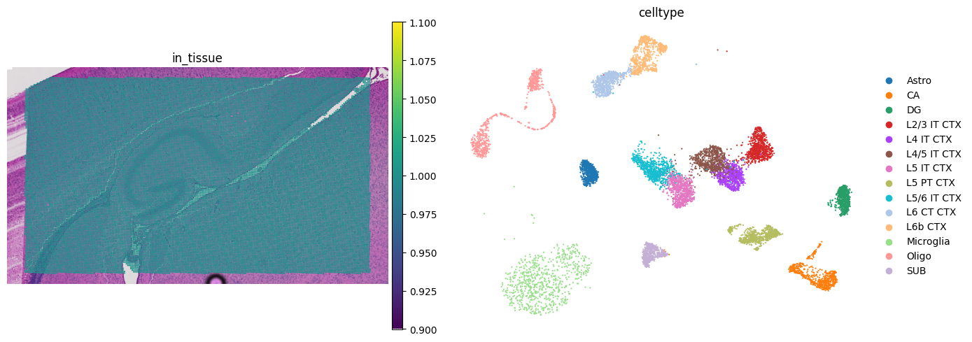
Verify all inputs carefully before proceeding.

fig, axs = mpl.pyplot.subplots(1, 2, figsize=(14, 5))
sc.pl.spatial(
    adata_st,
    color="in_tissue",
    frameon=False,
    show=False,
    ax=axs[0],
    img_key="hires",
)
sc.pl.umap(adata_sc, color=key_type, size=10, frameon=False, show=False, ax=axs[1])
mpl.pyplot.tight_layout()
mpl.pyplot.savefig(f"{results_folder}qc.jpg", bbox_inches="tight", dpi=400)

scatterplots.py (392): No data for colormapping provided via 'c'. Parameters 'cmap' will be ignored

Deconvolution: Marker Gene Selection and scRNA Reference Construction

Initialize the spatial transcriptomics and scRNA data. Specifically,

• adata_sc and adata_st are normalized

• cells and genes in adata_sc are filtered

• only the common genes shared by adata_sc and adata_st are kept

adata_sc, adata_st = spotiphy.initialization(adata_sc, adata_st, verbose=1)

Convert expression matrix to array: 0.8s
Normalization: 2.45s
Filtering: 1.68s
Find common genes: 0.01s

Select marker genes based on pairwise statistical tests. The selected marker genes are saved as a CSV file.

Users can adjust the following arguments:

• n_select: the maximum number of marker genes select for each cell type

• threshold_p: threshold of the \(p\)-value to be considered significant

• threshold_fold: threshold of the fold-change to be considered significant

• q: Since more than one \(p\)-values are obtained in using the pairwise tests, we only consider the \(p\)-value at quantile q. For additional details, please refer to the supplementary material of the paper.

• return_dict: Whether return a dictionary representing the marker genes selected for each cell type, or just return the list of all selected marker genes.

The parameters specified in the following code block provide a good starting point.

marker_gene_dict = spotiphy.sc_reference.marker_selection(
    adata_sc,
    key_type=key_type,
    return_dict=True,
    n_select=50,
    threshold_p=0.1,
    threshold_fold=1.5,
    q=0.15,
)
marker_gene = []
marker_gene_label = []
for type_ in type_list:
    marker_gene.extend(marker_gene_dict[type_])
    marker_gene_label.extend([type_] * len(marker_gene_dict[type_]))
marker_gene_df = pd.DataFrame({"gene": marker_gene, "label": marker_gene_label})
marker_gene_df.to_csv(f"{results_folder}marker_gene.csv")
# Filter scRNA and spatial matrices with marker genes
adata_sc_marker = adata_sc[:, marker_gene]
adata_st_marker = adata_st[:, marker_gene]

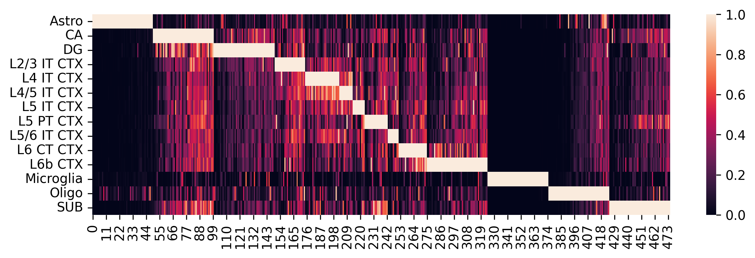
Construct the single-cell reference and visualize selected marker genes with heatmaps.

Adjust parameters in the previous step as needed to optimize marker gene selection:

• If several cell types are very similar (e.g., T cell subtypes), try setting q=0.3 or adjust accordingly.

• If there are limited marker genes for each cell type, try setting threshold_fold=1.2 or adjust as needed.

sc_ref = spotiphy.construct_sc_ref(adata_sc_marker, key_type=key_type)
spotiphy.sc_reference.plot_heatmap(
    adata_sc_marker, key_type, save=True, out_dir=results_folder
)

14it [00:00, 1216.12it/s]

Another opinion will be input your customized marker gene list. Use the following code:

#marker_gene = pd.read_csv(results_folder+'customized_marker_genes.csv', header=0)

Deconvolution: Cellular Proportion Estimation

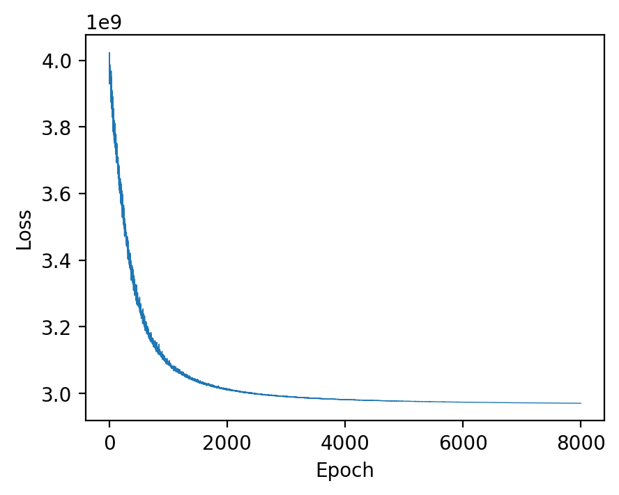
For performing the deconvolution, we calculate the posterior distribution of certain parameters within a probabilistic generative model using `Pyro <https://pyro.ai/>`__.

Parameters of the function estimation_proportion:

• X: Spatial transcriptomics data. n_spot*n_gene.

• adata_sc: scRNA data (Anndata).

• sc_ref: Single cell reference. n_type*n_gene.

• type_list: List of the cell types.

• key_type: Column name of the cell types in adata_sc.

• batch_prior: Parameter involved in the prior distribution of the batch effect factors. It is recommended to select from \([1, 2]\).

• n_epoch: Number of training epoch.

device = "cuda" if torch.cuda.is_available() else "cpu"
X = np.array(adata_st_marker.X)
cell_proportion = spotiphy.deconvolution.estimation_proportion(
    X,
    adata_sc_marker,
    sc_ref,
    type_list,
    key_type,
    n_epoch=8000,
    plot=True,
    batch_prior=1,
    device=device,
)
adata_st.obs[type_list] = cell_proportion
# Save the cellular proportions for future usage
np.save(f"{results_folder}proportion.npy", cell_proportion)
np.savetxt(f"{results_folder}proportion.csv", adata_st.obs[type_list], delimiter=",")

100%|██████████| 8000/8000 [04:05<00:00, 32.62it/s]

875694838.py (14): Trying to modify attribute `.obs` of view, initializing view as actual.

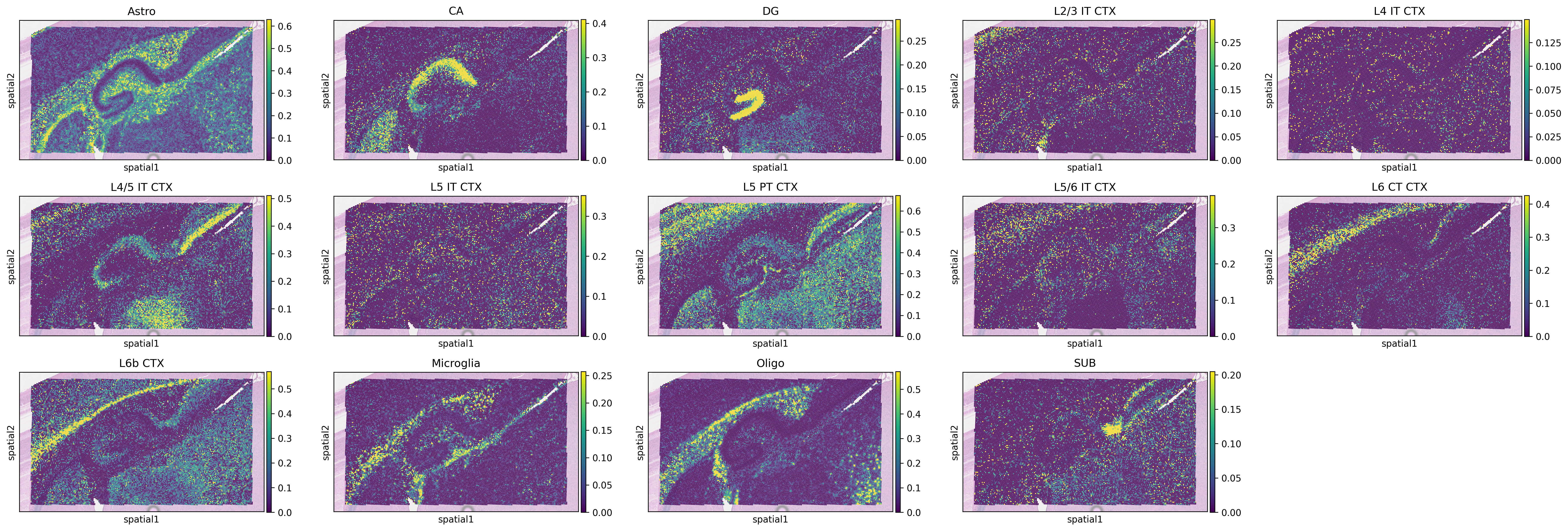
Generate heatmaps of cellular proportions.

vmax = np.quantile(adata_st.obs[type_list].values, 0.98, axis=0)
vmax[vmax < 0.05] = 0.05
with mpl.rc_context(
    {"figure.figsize": [5, 3], "figure.dpi": 300, "xtick.labelsize": 0}
):
    ax = sc.pl.spatial(
        adata_st,
        cmap="viridis",
        color=type_list,
        img_key="hires",
        vmin=0,
        vmax=list(vmax),
        show=False,
        ncols=5,
        alpha_img=0.4,
    )
    ax[0].get_figure().savefig(f"{results_folder}Spotiphy_deconvolution.jpg")